Numerical,Investigation,on,the,Deformation,of,the,Free,Interface,During,Water,Entry,and,Exit,of,a,Circular,Cylinder,by,Using,the,Immersed,Boundary-Multiphase,Lattice,Boltzmann,Flux,Solver

Guiyong Zhang,Haoran Yan,Hong Song,Heng Wang and Da Hui

Abstract In this work,the deformation of free interface during water entry and exit of a circular cylinder is investigated numerically by using the two-dimensional (2D) immersed boundary-multiphase lattice Boltzmann flux solver (IB-MLBFS). The fluid domain is discretized by finite volume discretization, and the flux on the grid interface is evaluated by lattice Boltzmann equations. Both the implicit velocity correction and the surface flux correction are implemented by using the immersed boundary-method to consider the fluid-structure interaction and the contact interface between the multiphase fluids and the structure.First,the water entry of a circular cylinder is simulated and the results are compared with the experiment,which considered the length-diameter ratio of the circular cylinder. The reliability of 2D simulation is verified and the deformation of the free interface is well investigated.Afterward,the water exit of a circular cylinder with constant velocity is simulated, which is less researched. In addition, the results show the advantage of present IB-MLBFS to some extent.Finally,the water exit and re-entry of a circular cylinder are presented,and the results present the complex deformation of the free interface and the dynamic response of the moving structure. Based on the numerical results, the free interface of the multiphase fluids is well captured, and the contact interface on the boundary of the moving structure is accurately presented by the IB-MLBFS.

Keywords Free interface;Water entry;Water exit;Immersed boundary method;Lattice Boltzmann flux solver

The interaction between multiphase fluids and structure in engineering is ubiquitous, in which the capture of the contact line between the multiphase fluids and the moving structure is challenging for numerical simulation.In investigating such problems, numerical methods for multiphase flows and the fluid-structure interaction are equivalently pivotal.

For the computational fluid dynamics in incompressible multiphase fluids, numerical methods can be classified into three categories based on different modeling such as the Navier-Stokes (N-S) solver in the macroscopic domain,the lattice Boltzmann method (LBM) in the mesoscopic domain, and the molecular dynamics (MD) in the microscopic domain.The N-S solvers are governed by mass conservation and momentum conservation on the macroscopic scale,which can be discretized with a high order of accuracy when the computational grids are sufficient. Hence, the N-S solver is considered the commonly used method in computational fluid dynamics, which has been widely developed for commercial applications.Different kinds of NS solvers have been developed and applied to engineering to investigate multiphase fluids. Bussmann et al. developed a three-dimensional volume tracking model, which was applied to the droplet impact onto a solid surface(Bussmann et al.1999,2000).Renardy et al.simulated moving contact line (MCL) problems using a volume-of-fluid method (Renardy et al. 2001). Nevertheless, for most N-S solvers, the computational efficiency is greatly affected by solving Poisson equations for pressure(Wang et al.2015a,d).Different from N-S solvers, the LBM is sourced from the kinetic theory and the governing equations can be solved directly in an explicit way. This feature ensures efficiency in computing and simplicity in programming and has led the LBM to be a popular method in recent decades(Guo et al. 2002; Mehravaran and Hannani 2008; Huang et al.2009b; Lee and Liu 2010; Zhou et al. 2012; Galindo-Torres et al. 2013; Lin et al. 2013; Galindo-Torres 2013;Galindo-Torres et al. 2016; de Rosis 2017;Yang et al.2018,2019;Chen et al.2020;Verdier et al.2020;Ru et al.2021;Wang et al.2021;Zhang et al.2021).Chen et al.developed an improved version of the simplified LBM(SLBM)(Chen et al.2017,2018;Chen and Shu 2020a,b).Based on their work, non-uniform meshes can be applied and non-Newtonian power-law fluid flows are investigated.The LBM has great advantages in efficiency, however,there exists a tie-up between the grid size and the time step,which results in the computation domain of the LBM being restricted to uniform mesh, and efficiency and accuracy may not be achieved simultaneously. In addressing the abovementioned challenge, a lattice Boltzmann flux solver(LBFS)has been developed by Wang et al.(2015b,c,2017, 2019b). In the LBFS, macroscopic property-conserved governing equations recovered by lattice Boltzmann equation (LBE) are discretized by cell-centered finite volume discretization (FVD). Different from other N-S solvers in which the inviscid and viscous fluxes on the cell interface are usually calculated separately, the LBFS reconstructs inviscid and viscous fluxes simultaneously by the local solution to the LBE.Given this feature,the LBFS removes the tie-up to allow its application to the non-uniform mesh and achieve accuracy, and the LBE in evaluating flux escapes from solving Poisson equations to achieve efficiency. Furthermore, Yang et al. (2020b, 2020a, 2021)developed LBFS in multiphase flow, and Chen et al.(2021) coupled the immersed boundary method (IBM)with LBFS in multiphase flow. Based on their work, the LBFS is well implemented and is proven to have wider application space in engineering.

Numerical methods can be classified into two categories based on different frames: the Lagrangian method and the Eulerian method. In investigating fluid-structure interactions (FSI) problems, implementing boundary conditions on the contact line between the structure and fluids remains a challenge (Shao et al. 2013). Thus, a body-fitted grid can be applied,where the grid is generated by concentrating the solid structure and sharing the same grid shape on the boundary line. This discretization of the computational domain ensures the boundary condition imposed with accurate solutions(Mittal and Iaccarino 2005).Nevertheless, generating body-fitted grids with good quality is challenging when the solid structure has a complex geometry, and the computational efficiency may be affected by the regeneration of grids when the solid structure is moving. In addressing the abovementioned drawbacks, nonbody conformal methods were presented (Peskin 1972;DeZeeuw and Powell 1993;LeVeque and Li 1994;Fedkiw et al. 1999; Liu et al. 2000; Li and Lai 2001; Lee and LeVeque 2003; Le et al. 2006), and the IBM, which is a feasible method, was presented by Peskin (2002). This method couples the Lagrangian method and Eulerian method, inheriting their advantages and removing the drawbacks to a certain extent.Wu and Shu(2009)developed an implicit velocity correction-based IBM, Shao et al. (2013)introduced the IBM to the contact line dynamic and Liu et al. (Liu and Ding 2015; Liu et al. 2017) introduced a diffuse-interface IBM for flows with MCLs. Previous research on the IBM has great importance to the multiphase fluids-structure interaction.

Previous work(Yan et al.2021,2022;Lu et al.2022)indicated that the LBFS is efficient and accurate to a certain degree compared with the LBM, which can be successfully implemented for the water entry and exit of rigid bodies(Xiao et al. 2022). In the present work, the IB-MLBFS was developed to investigate the deformation of the free interface during water entry and exit of a circular cylinder(Yan et al. 2022).The implicit velocity correction and surface flux correction are implemented by using IBM to consider the fluid-structure interaction and contact interface between the multiphase fluids and structure. In addition,Sun et al. (2018) developed an accurate and efficient smoothed particle hydrodynamics (SPH) model of the water entry of a circular cylinder. Wang et al. (2019a) improved the model with a novel non-reflecting boundary condition for fluid dynamics,and Sun et al.(2019)presented an investigation on the fully nonlinear water entry of a cone in the Stokes wave. The phenomena in the present simulation have been investigated experimentally by Wei and Hu (2014), Miao (1989), and Colicchio et al. (2009)and numerically by Zhang et al. (2017) with SPH, Zhu et al.(2007)with constrained interpolation profile(CIP),Colicchio et al. (2009) with ever set method (LSM), and Moshari et al.(2014)with the volume of fluid(VOF).The numerical results of the present IB-MLBFS indicate that the free interface deformation of multiphase fluids and the contact interface on the boundary of the moving structure are accurately simulated.The rest of this paper is organized as follows:Section 2 presents the methodology of the computational method and the detailed computation procedure,and Section 3 gives the conversion of units between the computational system and the physical system.The numerical investigation of the deformation of the free interface is presented in Section 4, and the conclusions are drawn in Section 5 at the end.

2.1 Multiphase lattice boltzmann flux solver

2.1.1 Governing equations

For the incompressible multiphase flow, the macroscopic N-S equations recovered by the multiphase lattice Boltzmann model can be written as follows(Wang et al.2015a):

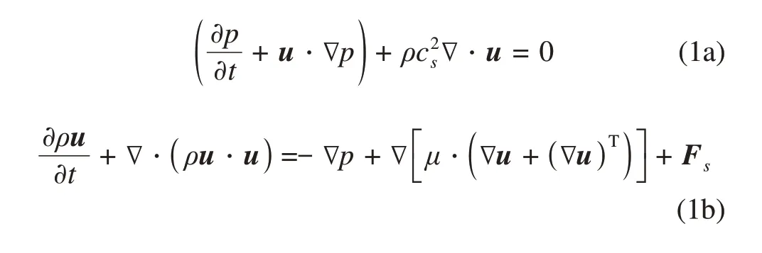
wherepis the pressure,uis the velocity,ρis the density,csis a constant related to the local sound speed,μis the dynamic viscosity, andFsis the surface tension force.The relationship between macroscopic properties and the lattice Boltzmann model has been establish, which can be written as follows:

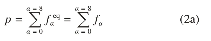
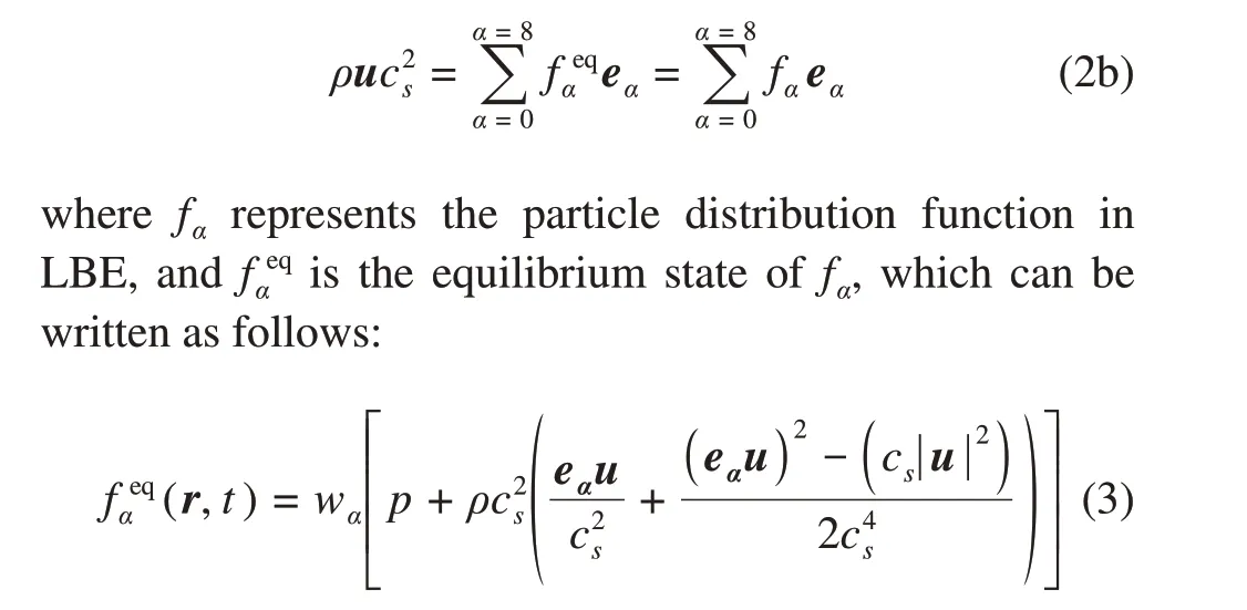
Then the connection between multiphase N-S equations and LBE is established.

2.1.2 Finite volume discretization

As an FVM-based flux solver, the fluxes at the cell interface between adjacent control cells must be evaluated.After establishing the connection between the N-S equation and LBE, the fluxes can be evaluated by reconstructing a lattice model locally at the cell interface(Figure 1).

For the whole fluids domain, implementing the FVD to Equation (1) over a control cell provides the following property-conserved equations:

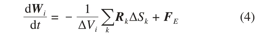
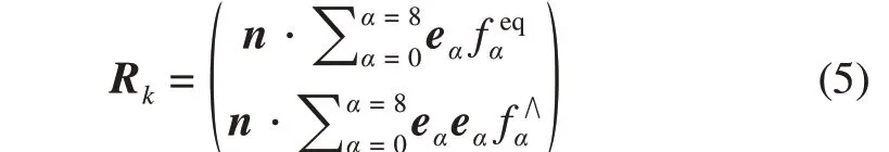
whereFEis the external force given by the source term such as the surface tension force, gravity, and boundary condition.Wi=(p,u) is the macroscopic variables of fluids in theith control cell.ΔVirepresents the volume of the control cell, and ΔSkrepresents the length/area of thekth interface enclosing the control cell for 2D/3D case. As shown in Figure 1, the fluxesRkare evaluated by reconstructing a lattice model locally at the cell interface.Rkcan be calculated as follows:

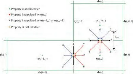
Figure 1 Evaluation of fluxes at the cell interface between adjacent non-uniform grid cells

In addition,the distribution functions in Equation(5)refer to the eight surrounding points in the lattice model.The propertiespanduof the surrounding points at(r-eαδt,t-δt)can be considered from that at(rt,t)by interpolation.

2.2 Correction by using the immersed boundary method

2.2.1 Implicit velocity correction

In the present work, the velocity of the flow field is initially predicted without considering the structure and then corrected by considering the solid boundary of the structure.The correction step modifies the velocity of the fluids based on the following relationship:

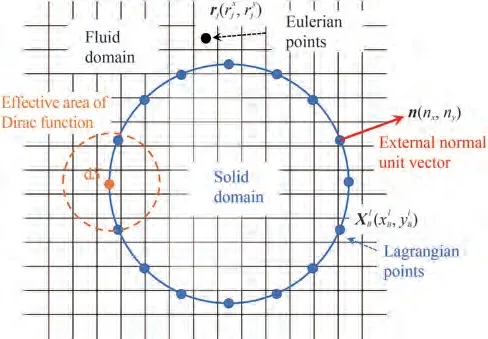
Figure 2 Illustration of the immersed boundary method

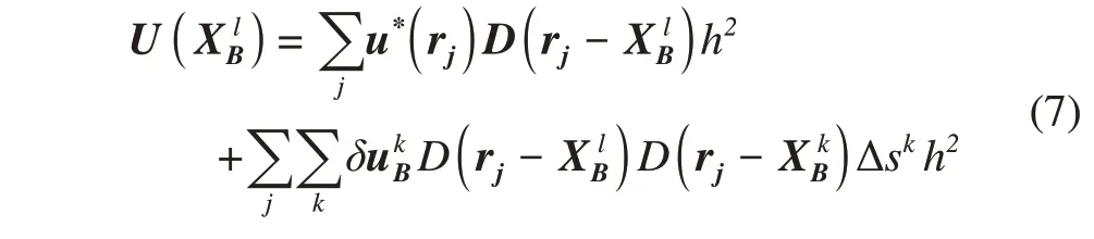
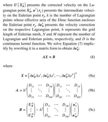
OnceδukBΔskare obtained, the velocity correction at each Eulerian point can be obtained using the following equation

Then, the correction can be performed on the whole flow field domain by Equation (6). In this work, the structure was motivated in the fluids thus theU(X lB)on all Lagrangian points is equal to the velocity of the cylinders.

2.2.2 Surface flux correction

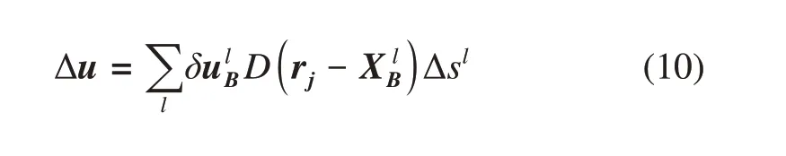
For multiphase flows, the densityρof fluids at the control cell can be determined by the heavy fluidρHand light fluidρL:

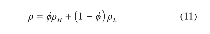
whereϕis the order parameter of the heavy fluids in the range of[0,1].In capturing the interface of the two immiscible fluids, the Cahn-Hilliard model was applied to computeϕ,and the conservative equation can be written as follows:

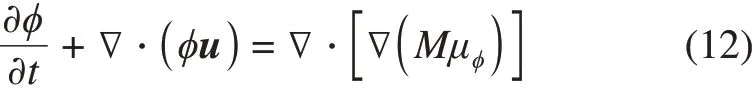
whereMis a constant which indicates the mobility;μϕis the chemical potential determined by the equilibrium state of the interface between fluid and fluid or fluid and structure. In the Cahn-Hilliard model, the boundary condition forϕis also determined by the material properties with a contact angleθeq,which is written as follows:

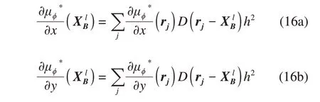
The Cahn-Hilliard only captures the interface of the two fluids henceϕandμϕare obtained without considering the structure. In illustrating the contact line between the boundary of the structure and the interface of multiphase fluids, theϕandμϕobtained by the Cahn-Hilliard model are defined as the intermediateϕ*andμϕ*,and then the surface flux correction is appended on the predicted intermediate properties of the fluids domain, which is similar to the velocity correction. Notably, for any Eulerian point in the effective area of the Dirac function (Figure 2), its control volume must enclose a small surface area. For this case, the surface fluxes from two opposite directions will contribute positively toϕin the control volume. In obtaining the surface flux correction, we initially calculate the derivative on the solid boundary by using the following interpolation formula:

Then the normal derivative at the boundary point can be illustrated as:

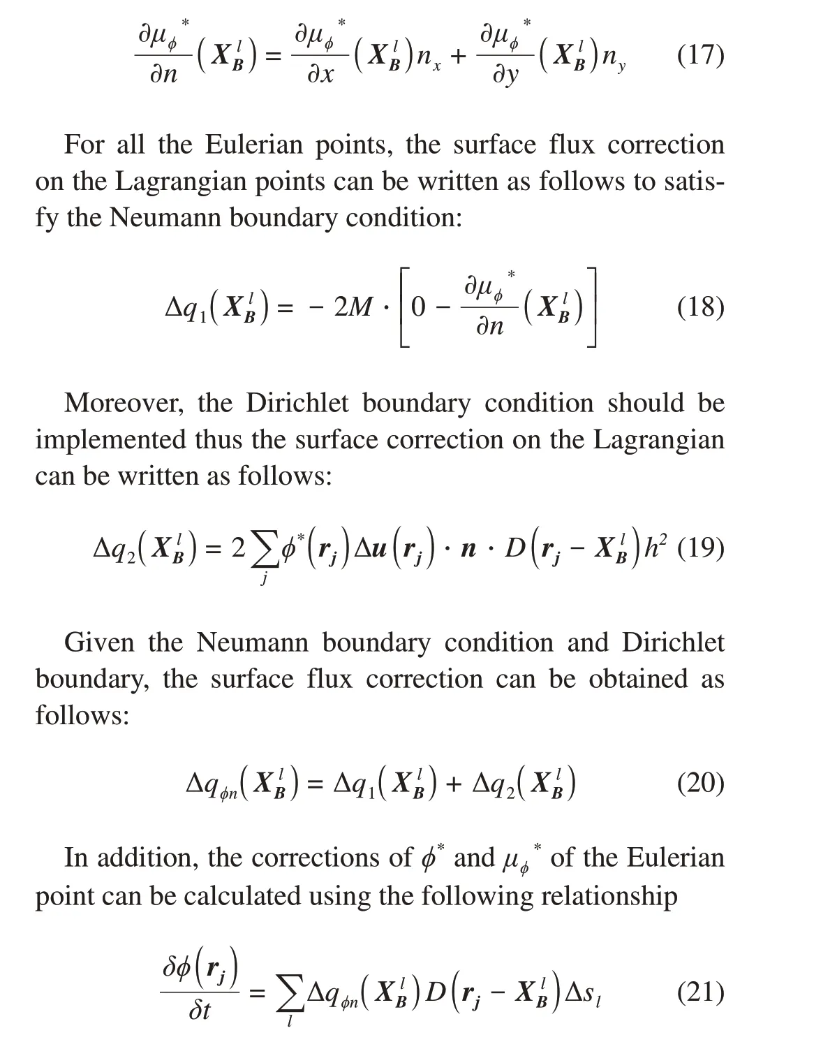
Afterward, the order parameterϕcan be finally corrected using the following equation:

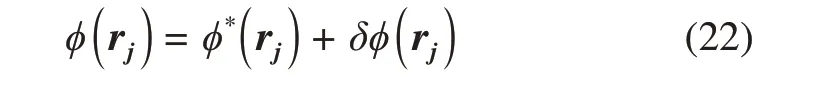
Then, the whole fluid domain has been corrected by the Dirichlet boundary condition and Neumann boundary condition

2.3 Rigid body dynamics

In the IBM, the inertial or internal mass effects of the structure exist, which may influence the accuracy (Shukla et al. 2007). The flow field within the structure boundary is set as the light fluid to minimize these effects, whose density is 0.001 times that of the heavy fluid, and the noslip boundary is applied at the surface of the structure.The two-dimensional Newton-Euler equations, which describe the rigid body motion,can be written as follows:

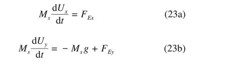
whereFEis the external force on the rigid body generated by the surrounding multiphase flows, which can be calculated on the basis of the pressure acting on the structure boundary using the following equation:

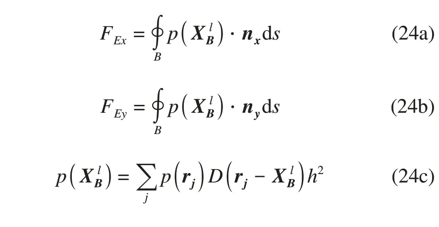
Using the obtained forces calculated by Equation (20),the motion and velocity of the rigid body can be computed and updated through Equation(19),and then the MCL can be corrected

2.4 Sequence of computation

1) Predict the fluid domain by solving Equation (4) and obtain the intermediate volume factor and intermediate velocity(Section 2.1).

2)Correct the velocity by using the IBM using Equation(10)(Section 2.2.1).

3) Correct the volume factor by using the IBM using Equation(22)(Section 2.2.2).

4)Compute the external force acting on the structure by Equation (24), and then update the location of the moving structure(Section 2.3).

5) Repeat 1 to 4 until the desired iteration number is reached.

For the numerical simulation,all the properties are computed in non-dimensional forms by using a computer.When examining the numerical results with physical experiments, the properties in the LBFS system should be the same as that in the physical system.The conversion of units is conducted as follows to build the connection between the numerical simulation and physical experiment.LetL′,M′andT′be the ratios of length,mass,and time,respectively,between the LBFS system and physical system,the conversion formula can be written as follows,and their values are set(Table 1).

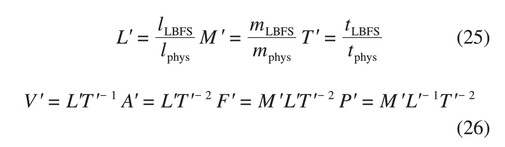
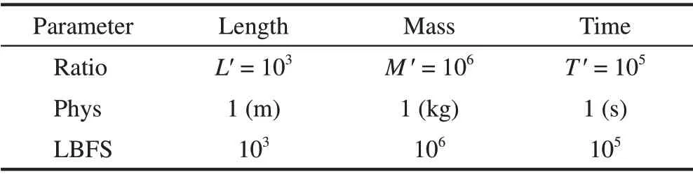
Table 1 Ratios and values of the basic quantities

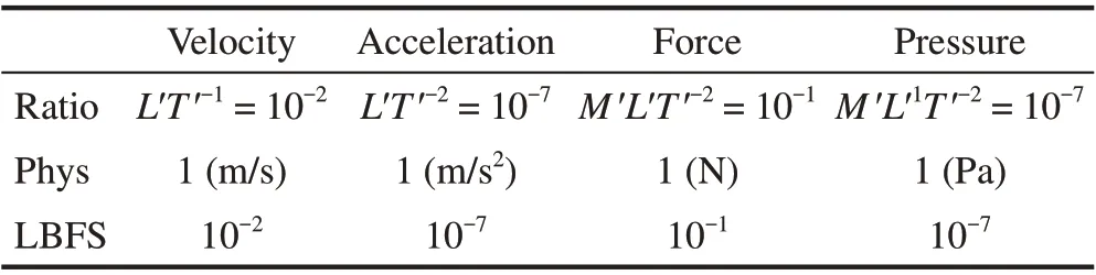
Table 2 Ratios and values of the derived quantities

Using the abovementioned relationship, the properties in the physical system can be clearly converted to the respective numerical values in LBFS, hence, the obtained numerical results can be conducted to the physical system,which ensures the implementation of LBFS in engineering.

In this section, the numerical simulations of water entry and exit are presented. The deformation of the free interface is clearly illustrated and the results are compared with experiments.For all the cases,the grid size is set as 10-3m and the time step is set as 10-5s.The mobility in the Cahn-Hilliard model is set asM= 20.0, and the grid size ratio between Lagrangian point and Eulerian point is set as 1.0,which has been proven to be suitable values to ensure efficiency and accuracy (Huang et al. 2009a; Wang et al.2015b;Chen et al.2020;Yan et al.2021,2022).The density of the light gaseous fluid is set asρL= 1 kg/m3,whereas that of the heavy liquid fluid is set asρH= 1 000 kg/m3.Moreover, the dynamic viscosity ratio of the liquid fluid and gaseous fluid is defined asμH/μL= 100.

4.1 Water entry of a free circular cylinder

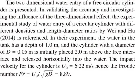
For numerical simulations, the fluid domain is set as 16D× 30D, and the initial acceleration of the structure in the gaseous fluid is partly simplified, that is, the cylinder is posited near the free-surface with velocity at the beginning to improve the computational efficiency (Figure 3). The cylinders with densities ofρs= 1 370 kg/m3andρs= 900 kg/m3are defined similarly to the experiment. The bounce-back boundary condition is applied to the both sides and the bottom, and the pressure-outlet boundary condition is applied to the top boundary.The moment when the cylinder touches the free interface is defined ast= 0.

Figure 4 demonstrates the water entry by experiment(Wei and Hu 2014) and the IB-MLBFS at respective times, and the cylinder has a density ofρs= 1 370 kg/m3andL/D= 4.The development of jets from both sides, the inversion of the cavity shape above the cylinder, and the contact interface surrounding the cylinder are consistent.The surface tension force acting on the free interface maintains the cavity shape,and the cavity is develops with time as the Froude number is large enough.For a detailed illustration, Figure 5 shows the contact interface of the cylinder boundary, gaseous fluid, and liquid fluid. The thickness of the free interface, which maintains the two fluids immiscible by surface tension, is clearly described. In addition, the solid boundary of the cylinder is indicated by dashed lines with no specific color filled inside,hence,the contact line between the structure and multiphase fluids is evident. This feature indicates that the order parameter is well conserved on the solid boundary as the convective and diffusive terms are corrected by the surface flux correction. Moreover, the 2D simulation can represent the phenomenon atL/D= 4.The results show that the present IB-MLBFS satisfies the conserved law on the interface,which can deal with a moving boundary.

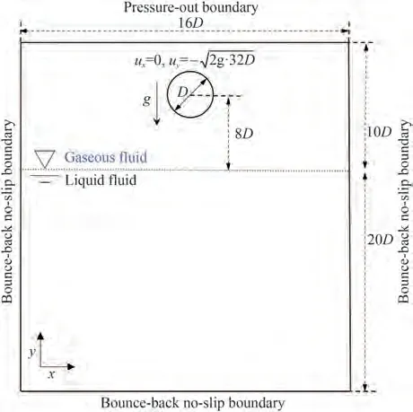
Figure 3 Computational domain of water entry of a free circular cylinder

Figure 4 Evolution of the water entry of a circular cylinder a density of ρs = 1 370 kg/m3 at respective times

When the cylinder has a lower densityρs= 900 kg/m3than the liquid fluid, the pressure acting on the structure and viscosity of the fluids are considerable, hence, the deformation of the free interface may be different from the abovementioned results.As shown in Figure 6, the evolution of the water entry of a circular cylinder with a density ofρs= 900 kg/m3is simulated by the current IB-MLBFS.Compared with the results shown in Figure 4, whereρs=1 370 kg/m3, the cavity shape is nearly the same whent≤74 ms, but the inversion of the cavity shape in the present simulation appears earlier, hence, the deformation of the free interface is quite different att= 120 ms, and the displacement of the cylinder is shorter. This result can be attributed to the small Froude number in the present case,thus gravity can perform an effective influence on the deformation of the free interface.Nonetheless,the cavity can be observed clearly, and the shape is significant, which indicates that the surface tension force acting on the free interface greatly maintains the contact line among the multiphase fluids.In investigating the influence on the deformation of the free interface by the length-diameter ratio, the instantaneous snapshots att= 101 ms by the present 2D simulation and experiments(Wei and Hu 2014)with different length-diameter ratios are shown in Figure 7.The comparison shows that the cavity width increases and the jet spreads to both sides with the increase of the length of the cylinder. Notably, the deformation of the free interface in the present 2D simulation results is close to that of the experimental results ofL/D= 4, and the comparison of the depth of penetration between the present IB-MLBFS and experiments is shown in Figure 8.The abovementioned results indicate that the length-diameter ratio plays a pivotal rule in the deformation of the free interface, and the 2D simulation is considerable only when the length-diameter ratio is large.Nonetheless,the 2D simulation can accurately predict the displacement of the circular cylinder to a certain extent without the influence of the length-diameter ratio,particularly whenρs= 900 kg/m3.

4.2 Water exit of a circular cylinder with constant velocity

Compared with water entry, the water exit has been less researched. Therefore, the viscosity, gravity, and surface tension of multiphase fluids are particularly important,which lead to the complex deformation shape of the free interface.The abovementioned parameters require the high accuracy of the numerical solver to evaluate the pressure and volume factor. In this section, the 2D water exit of a circular cylinder with constant velocity is presented by IBMLBFS, which has been investigated experimentally by Miao (1989) and simulated numerically by Zhang et al.(2017),Zhu et al.(2007),and Xiao et al.(2022).This case is characterized by the Froude numberFr=v/ 2gr,wherevis the absolute value of the constant velocity in the vertical direction.Based on the experiment,two different Froude numbers,Fr= 0.764 4 andFr= 0.462 7, were investigated. The circular cylinder is initially posited under the free interface with the distance between the top of the cylinder and the mean free interface isvt r= -5.5, which reaches the desired constant velocityvafter a temporary acceleration at the positionvt r= -5.0. In the present simulation,the Reynolds numberRe= 2ρHvr/μHwas set similar to that of previous research and defined as 1 000.The computational domain was set as 10D× 10D, and bounce-back boundary condition was applied on the left, right, and bottom sides, whereas the pressure-outlet boundary condition was applied on the top. Instantaneous contours of pressure and density were printed and compared with other numerical solvers, and the coefficient of the vertical forceCe=Fy/ρv2rwas presented to compare with experimental and other numerical solvers.

Figure 5 Detailed instantaneous density contours near the interface at t = 74 ms.The dashed line indicates the solid boundary of the cylinder,which is presented by Lagrangian grid points

Figure 6 Instantaneous density contours of water entry of a circular cylinder a density of ρs = 900 kg/m3 at respective times by the current IB-MLBFS

Figure 7 Snapshots of the water entry of a circular cylinder with ρs = 900 kg/m3 by the IB-MLBFS and experiments:(a)(b)t = 101 ms,(c)t =100 ms,(d)t = 96 ms

Figure 8 Comparison of the penetration depth between the current IB-MLBFS and experiments

Figure 9 shows the evolution of fluid pressure and deformation of the free interface withFr= 0.764 4 by SPH(Zhang et al. 2017), CIP (Zhu et al. 2007), and current IB-MLBFS. Evidently, a good agreement is achieved. As shown in Figure 9(a) and Figure 9(b), two regions of the fluid can be observed below the cylinder where the pressure is significantly lower than the surrounding fluid domain,and this phenomenon can still be observed atvt r= 2 by the IB-MLBFS (Figure 9(b)) but not by SPH (Figure 9(a)).By comparing Figure 9(c) and Figure 9(d), the thickness of the liquid fluid layer and the deformation of the free interface surrounding the cylinder are nearly the same. Nevertheless,the free interface and contact interface of the cylinder presented by the IB-MLBFS in Figure 9(d) show clear deformation because of the surface tension force and surface tension flux correction. Moreover, the fluid layer shown in Figure 9(c) is enclosed because the structure and thickness of the free interface are thick, whereas the layer by the present method shown in Figure 9(d) is conserved well on the solid boundary. Furthermore, the thickness of the free interface is thin enough to represent the detailed deformation.

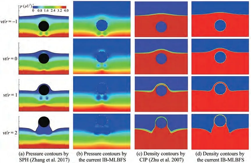
Figure 9 Comparison of instantaneous contours of water exit of a circular cylinder with constant velocity and Fr = 0.764 4 at respective times

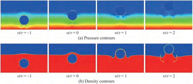
Figure 10 Instantaneous contours of water exit of a circular with constant velocity by present IB-MLBFS at respective times,Fr = 0.462 7

ForFr= 0.462 7, the gravity and viscosity of the liquid fluid can lead to a complex free interface (Figure 10).Although the fluid below the cylinder still exits two regions with lower pressure, the difference in the pressure is less.For the deformation of the free interface,compared with the results shown in Figure 9, the thickness of the fluid layer above the cylinder is less atvt/r= 0 whenFr= 0.462 7,and then it can hardly maintain but slide to the two sides atvt/r= 1, as the gravity is predominant, and less liquid fluid is lifted atvt/r= 2.As shown in Figure 10(b), two jets appear on the free interface and the gaseous fluid is observed under the free interface, which indicates that the gaseous fluid is mixed with liquid fluid and complex deformation may occur. In investigating this deformation, the detailed density contour atvt/r= 1.5 is shown in Figure 11.Two narrow gaseous gaps are generated on both sides of fluids below the cylinder because the liquid fluid lifted by the cylinder drops, whereas that from each side moves to the middle, and it does not occur atvt/r= 2 (Figure 9(d))because the viscosity of the fluid is predominant rather than the gravity at that time underFr= 0.764 4.Apart from the deformation of the free interface, the time domainCeunder the two different Froude numbers are plotted in Figure 12. Comparing present results with experimental results, the trend of the results by the IBMLBFS is highly consistent with that of the experimental results over time.The amplitude ofCepredicted by the IBMLBFS is close to that predicted by other numerical methods. AlthoughCeobtained by other solvers are smooth curves,the IB-MLBFS can successfully predict the oscillation curve ofCewith time,which is consistent with the experimental results.

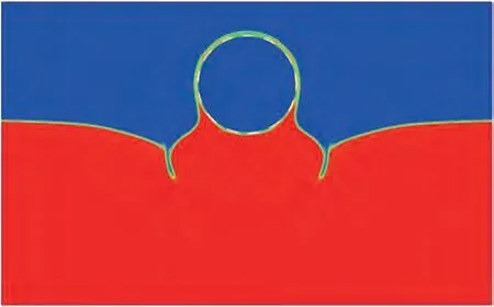
Figure 11 Density contour of the water exit of a circular cylinder with a constant velocity at vt/r = 1.5 by the current IB-MLBFS,Fr =0.462 7

4.3 Water exit and re-entry of a free circular cylinder

In this section, the water exit and re-entry of a free circular cylinder are presented. Different from water exit with constant velocity, the cylinder in this section is free from gravity, which interacts with fluid dynamically. Once the cylinder is lighter than the heavy fluid and fully submerged under the free interface, the cylinder moves up as it accelerates from a static state under buoyancy and partly exits the free interface as the pressure is predominant.Afterward, it slows down and reaches the summit under the predominant gravity, and finally drops down and re-enters the water. This procedure may repeat several times until the cylinder finally reaches a static state because of the viscosity of the fluids, and the complex deformation of the free interface requires computational stability and accuracy in capturing the contact interface between the multiphase fluids and moving solid structure for the numerical solver. Colicchio et al. (2009) studied the phenomenon by experiment and LSM, and Moshari et al. (2014) represented a numerical study by VOF. The abovementioned solvers successfully simulated the water exit of a free circular cylinder, and the results were consistent with the experiment. Nonetheless, the water re-entry phase has not been well simulated because of the complex deformation shape of the free interface. In this section, the phenomenon obtained by the experiment is represented by the IB-MLBFS.The cylinder,with a density of 0.62 times that of water and a diameter of 0.3 m,is fully submerged with its center at a depth of 0.46 m from the undisturbed free interface. The computational domain is set as 9D× 7D, and the bounceback boundary condition is applied on the left, right and bottom sides of the tank,whereas the pressure-outlet boundary condition is applied on the top.

The pressure and density contours for the evolution of water exit and re-entry of a circular cylinder at time 0.25 s ≤t≤2.00 s are illustrated in Figure 13 and Figure 14,respectively. Figure 15 shows the time-domain displacement and velocity of the cylinder from water exit to water re-entry. The deformation of the free interface and the hydrodynamic response of the cylinder are clearly demonstrated. In the present simulation results, the cylinder accelerates to the maximum velocity att= 0.69 s, meanwhile, the fluids are driven with velocity. Hence, the pressure under the cylinder is greater than that at other times(Figure 13(c)). Then, it reaches the summit att= 0.95 s,and the fluids lifted by the cylinder have dropped and collide with the fluids coming from each side, which leads to complex deformation of the free interface (Figure 14(d)).Afterward, the cylinder drops with the fluids surrounding it, re-enters the water, separates the fluids below to each side,and reaches the lowest depth att= 1.51 s(Figure 14(f)and Figure 13(f)). In this procedure, the two regions with lower pressure are formed because the fluids slide from the cylinder and move to the sides. Notably, the separated liquid fluid moves back to the middle and climbs up to the surface of the cylinder att= 1.75 s (Figure 14 (g)), and then slides down again when the cylinder moves up under buoyancy(Figure 14(h)).This simulation shows the stability and accuracy of the IB-MLBFS as the buoyancy acting on the cylinder is generated by the pressure of the fluids and the complex deformation of the free interface is well captured on the moving boundary of the structure.

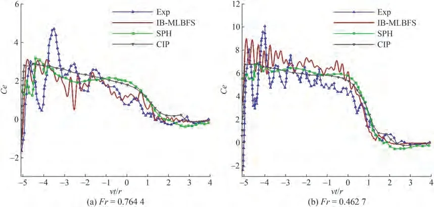
Figure 12 Comparison of the coefficient of the vertical force of the cylinder among the current IB-MLBFS, SPH (Zhang et al. 2017), CIP(Zhu et al.2007),and experiment(Miao 1989)

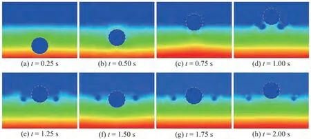
Figure 13 Evolution of pressure contours of the water exit and re-entry of a free circular cylinder at respective times

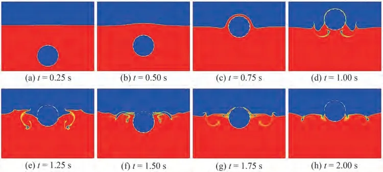
Figure 14 Evolution of density contours of the water exit and re-entry of a free circular cylinder at respective times

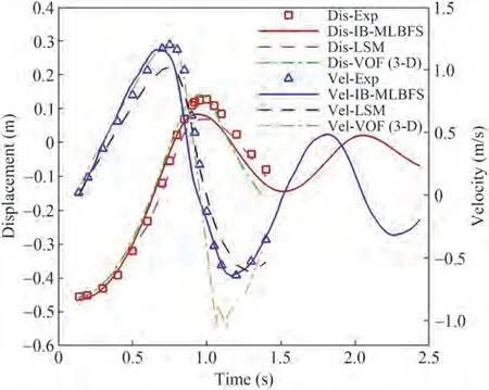
Figure 15 Comparison of the displacement and velocity of the cylinder between the current IB-MLBFS and experiment

In this work, the deformation of the free interface during water entry and exit of a circular cylinder was investigated numerically by the IB-MLBFS. Implementing the IBM, the implicit velocity correction and surface flux correction were appended to the LBFS,hence,the IB-MLBFS can deal with the multiphase fluids-structure interaction.The accuracy of the solver was validated and the numerical simulation was well represented.

First,the simulation of water entry of a circular cylinder was presented. The reliability of 2D simulation was verified by comparing with experiment which considered different length-diameter ratios, and the deformation of the free interface was investigated. Then, the less-researched water exit of a circular cylinder with constant velocity was simulated. By considering different Froude numbers, the deformation of the free interface was investigated and the influence of gravity,viscosity and velocity was studied.Finally,the water exit and re-entry of a free circular cylinder were simulated.The complex deformation of the free interface and hydrodynamic response of the cylinder were well investigated, and all the numerical results were consistent with the experiments.The IB-MLBFS not only successfully simulated the complex phenomena but also achieved accuracy and stability to a certain extent compared with other solvers.

In this work,only the circular shape of the moving structure was considered,and the collision and rotation were ignored because the present work focused on the free interface of the fluid domain. Moreover, the present solver is direct numerical simulation, which can hardly apply coarse mehes to a high Reynolds number phenomena,such as the turbulent flow.Future work may introduce the Large Eddy Simulation to the IB-MLBFS and apply the current solver to interacting multi-structures and complex shapes,which may lead to the wider application of the solver in engineering.

FundingSupported by the National Natural Science Foundation of China (52061135107), the Fundamental Research Fund for the Central Universities (DUT20TD108, DUT20LAB308), the Liao Ning Revitalization Talents Program(XLYC1908027),and Dalian Innovation Research Team in Key Areas(2020RT03).

Open AccessThis article is licensed under a Creative Commons Attribution 4.0 International License, which permits use, sharing,adaptation, distribution and reproduction in any medium or format,as long as you give appropriate credit to the original author(s) and thesource, provide a link to the Creative Commons licence, and indicateif changes were made. The images or other third party material in thisarticle are included in the article’s Creative Commons licence, unlessindicated otherwise in a credit line to the material. If material is notincluded in the article’s Creative Commons licence and your intendeduse is not permitted by statutory regulation or exceeds the permitteduse, you will need to obtain permission directly from the copyrightholder.To view a copy of this licence,visit http:/creativecommons.org/licenses/by/4.0/.

推荐访问:water Interface Exit